15 — Scaling, Performance, Cost & Reliability Engineering

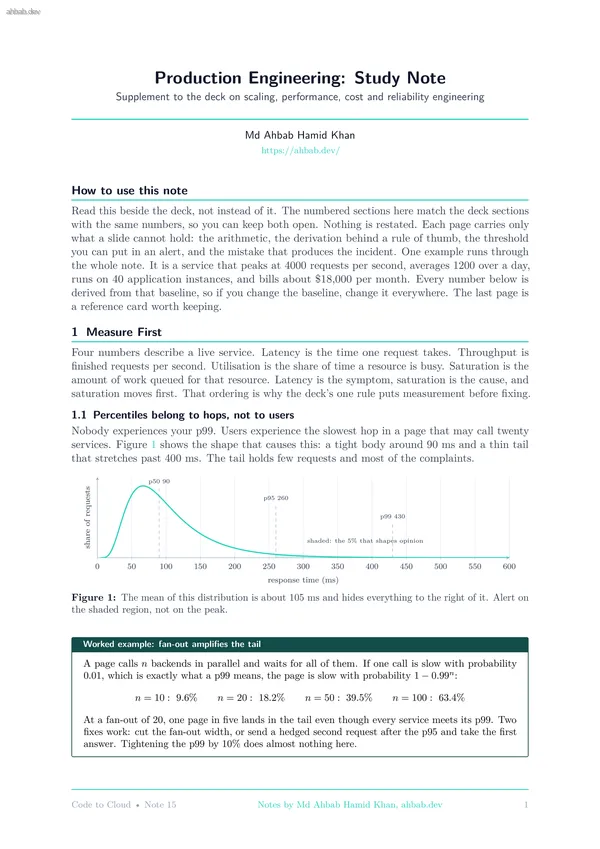
Production Engineering: Study Note Supplement to the deck on scaling, performance, cost and reliability engineering Md Ahbab Hamid Khan https://ahbab.dev/ How to use this note Read this beside the deck, not instead of it. The numbered sections here match the deck sections with the same numbers, so you can keep both open. Nothing is restated. Each page carries only what a slide cannot hold: the arithmetic, the derivation behind a rule of thumb, the threshold you can put in an alert, and the mistake that produces the incident. One example runs through the whole note. It is a service that peaks at 4000 requests per second, averages 1200 over a day, runs on 40 application instances, and bills about $18,000 per month. Every number below is derived from that baseline, so if you change the baseline, change it everywhere. The last page is a reference card worth keeping. 1 Measure First Four numbers describe a live service. Latency is the time one request takes. Throughput is finished requests per second. Utilisation is the share of time a resource is busy. Saturation is the amount of work queued for that resource. Latency is the symptom, saturation is the cause, and saturation moves first.

Worked example: Little’s Law sizing a thread pool Little’s Law says L = λW, where L is the number of requests inside the system, λ the arrival rate and W the time each one spends inside. At peak, λ = 4000 per second and W = 25 ms: L = 4000 × 0.025 = 100 requests in flight. Spread over 40 instances that is 2.5 busy threads each, so a pool of 8 per instance has room to spare. Now a downstream dependency slows from 25 ms to 200 ms. Nothing else changed: L = 4000 × 0.2 = 800, thatis 20 per instance. The pool of 8 is now the limit, requests queue in front of it, and the queue wait is added to every response. Pools rarely break when traffic rises. They break when W rises. Size pools from λW at the worst W you are willing to serve, then set a queue limit and shed load past it. 1.2 Error budgets in minutes you can feel An SLO is a target for an SLI, and the error budget is the part of the month you are allowed to miss it. Percentages are hard to argue with. Minutes are not. Table 1 converts the usual targets, and the last column is the one to quote when somebody asks for one more nine. Table 1: Error budget in real minutes, on a 30 day month of 43,200 minutes. At 99.95 percent a single 20

2.1 Why closed-loop clients hide the tail A closed-loop client keeps a fixed number of virtual users, and each one waits for its own response before sending the next request. When the server stalls, the client stops sending. The requests that should have arrived during the stall are never issued, so they are never timed. That gap is coordinated omission, and Figure 2 shows it. An open model sends at a fixed rate no matter what the server does, so the delay lands in the numbers where it belongs. server stalled 2 s closed loop no requests sent, nothing measured open model requests keep arriving and queue, so the wait is recorded Figure 2: The same stall, measured two ways. The closed-loop run reports one slow request. The open-model run reports 200 of them, which is what the users on the other side of the stall actually saw. Worked example: what omission does to a p99 A test plans one request every 10 ms for 100 s, so 10,000 requests. Normal responses are near 20 ms. At t = 50 s the server stalls for 2 s. • Closed loop: 9,800 fast samples plus one 2000 ms sample. The p99 is the 100th slowest sample, which is still about 30 ms. The report says the service is healthy. • Open model: the