Gene Prediction, Genome Annotation and Genome Browsers

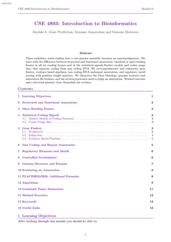
CSE 4893 Introduction to Bioinformatics Module 6 CSE 4893: Introduction to Bioinformatics Module 6: Gene Prediction, Genome Annotation and Genome Browsers Abstract These subsidiary notes explain how a raw genome assembly becomes an annotatedgenome. We start with the difference between structural and functional annotation, thenlook at open reading frames in all six reading frames and at the statistical signals,Markov models and codon usage bias, that separate coding from non coding DNA. We surveyprokaryotic and eukaryotic gene finders, evidence based pipelines, non coding RNA andrepeat annotation, and regulatory motif scoring with position weight matrices. We thencover the Gene Ontology, genome browsers and annotation file formats, and the accuracymeasures used to judge an annotation. Worked exercises and a keyword glossary close themodule for revision. Contents 1 Learning Objectives 1 2 Structural and Functional Annotation 2 3 Open Reading Frames 2 4 Statistical Coding Signals 3 4.1 Markov Models of Coding Potential . . . . . . . . . . . . . . . . . . . . . . . . . . . . . . . . 3 4.2 Codon Usage Bias . . . . . . . . . . . . . . . . . . . . . . . . . . . . . . . . . . . . . . . . .

CSE 4893 Introduction to Bioinformatics Module 6 1. Distinguish structural annotation from functional annotation and name the output each one produces. 2. Enumerate the six reading frames of a DNA sequence and find the open reading frames within them. 3. Explain how Markov models and codon usage bias give a log odds measure of coding potential. 4. Compare prokaryotic gene finders with generalised hidden Markov model and evidence based eukaryotic pipelines. 5. Score a motif with a position weight matrix, read GFF3, BED and VCF records, and evaluate an annotation at base and exon level. 2 Structural and Functional Annotation Annotation is the act of adding meaning to an assembly. It happens in two layers that areeasy to confuse, so we define them carefully before going further. Two layers of annotation Structural annotation answers where. It places coordinates on the assemblyfor genes, tran- scripts, exons, coding sequences, non coding RNAs and repeats. Functional annotation answers what for. It attaches biological meaning tothose features, for example a protein family, a Gene Ontology term, an enzymenumber or a pathway membership. Both layers are versioned. A gene model that was cor

CSE 4893 Introduction to Bioinformatics Module 6 +1 +2 +3 −1 −2 −3 longest ORF position on the contig Figure 1: The six reading frames of one contig. Each bar is a stop free stretch. The longestopen reading frame, here in frame +3, is highlighted and would be the first candidategene to test. Finding an ORF is only the first step. We still need a numerical statement of how codinglike a stretch of DNA looks. Two signals do most of the work: the local compositioncaptured by Markov models, and the skewed use of synonymous codons. 4.1 Markov Models of Coding Potential Train one model on known coding sequence and one on known non coding sequence, then compare- how well each explains a candidate window. The comparison is a sum of log odds. Coding potential as a log odds score S(x) = X i log2 Pcod(xi | x i−1 i−k ) Pnon(xi | x i−1 i−k ) A positive S(x) favours the coding model, a negative S(x) favours the non coding model,and the units are bits. Training. Conditional probabilities are counted from a trusted set of genes. For ak th order model over four bases we need 4k+1 counts, so a fifth order model alreadyneeds 4096 parameters per frame. Coding models are usually three periodic, thatis,